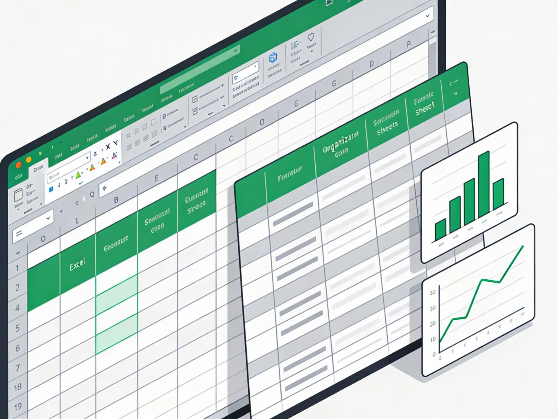
Spreadsheets & Data: Beginner's Blog Tutorial

Most spreadsheets start as a quick note and grow into a mess nobody trusts. This tutorial walks you from a messy sheet to a clear answer: how to structure your data as one clean table, which formulas cover ninety percent of everyday work, what a pivot table actually does, and how to build a chart that answers a real question. Everything here works the same way in Excel and Google Sheets.

Step 1: Put everything in one flat table

Almost every spreadsheet problem traces back to layout. Merged cells, subtotal rows mixed into the data, one tab per month, colors that carry meaning: all of these make formulas and pivot tables harder than they need to be. The fix is one flat table with a simple contract:

• Row 1 contains headers, one short unique name per column.
• Every row below it is one record: one order, one expense, one measurement.
• Every column holds one kind of value: a date column holds only dates, an amount column only numbers.
• No blank rows, no subtotal rows inside the data, no merged cells.

If your current sheet has monthly tabs, add a Month column instead and stack everything into one table. It feels like a step backwards because you lose the visual grouping. It is not: totals per month become a single formula or pivot table, and adding a new month means adding rows, not rebuilding formulas.

One more habit that pays off: keep raw data and calculations on separate tabs. The data tab is only for records. Summaries, formulas and charts live elsewhere and point at the data. That way you can paste in new rows without breaking anything.

Step 2: Learn the four formulas that do most of the work

You do not need hundreds of functions. Four families cover most daily questions.

SUM and AVERAGE total or average a range: =SUM(C2:C200), =AVERAGE(C2:C200). Their conditional versions are more useful in practice: =SUMIF(B2:B200,"Groceries",C2:C200) adds only the amounts where column B says Groceries. SUMIFS, COUNTIFS and AVERAGEIFS accept multiple conditions, for example a category and a month at the same time.

IF makes a decision per row: =IF(C2>100,"review","ok") returns one value when the test is true and another when it is false. You can nest IFs, but if you find yourself three levels deep, a lookup table is usually the cleaner tool.

VLOOKUP fetches a matching value from another table. =VLOOKUP(A2,Products!A:C,3,FALSE) searches for the value of A2 in the first column of the range and returns the value from the third column of that range. Two classic pitfalls: always end with FALSE so you get exact matches only, and remember that VLOOKUP can only look to the right of the column it searches in.

XLOOKUP is the modern replacement and available in current versions of both Excel and Google Sheets: =XLOOKUP(A2,Products!A:A,Products!C:C). You name the lookup column and the return column separately, so the right-only limitation disappears, it defaults to exact match, and it takes an optional fourth argument for what to show when nothing matches. If it is available to you, prefer it.

Step 3: Clean the data before you calculate

Formulas are only as good as the cells they read. Before you trust a total, spend ten minutes on hygiene:

1. Turn on the filter on your header row and open each column's filter list. It shows every distinct value, so typos like "groceries", "Groceries " and "Grocery" jump out immediately.
2. Use =TRIM(A2) to strip stray spaces, which are the most common reason a lookup "mysteriously" fails.
3. Check that numbers are numbers. Values aligned to the left are usually text; a SUM over them quietly returns a lower total than the real one because the text values count as nothing.
4. Remove duplicates with the built-in tool (Data menu in both Excel and Google Sheets), but check first whether duplicates are errors or legitimate repeated records.

The honest expectation: cleaning is most of the work. A question that takes thirty seconds to answer on clean data can take an afternoon on a dirty sheet.

Step 4: Pivot tables, in plain words

A pivot table is a summary machine. You point it at your flat table and answer three questions: what do I want to group by (rows), what do I want to split it by (columns, optional), and what do I want to calculate (values). The spreadsheet then does all the grouping and totalling for you, with no formulas.

Example: a table of expenses with columns Date, Category and Amount. Drag Category into rows and Amount into values, and you have a total per category. Add Month to columns and you have a category-by-month grid. Change the value calculation from sum to count or average with two clicks.

Three things beginners trip over:

• A pivot table does not update itself when you add rows below the original range. Refresh it, or better, base it on an entire-column range or a proper Excel table so new rows are picked up.
• If a category shows up twice in the pivot, the source data has two spellings. Fix the data, not the pivot.
• The value defaults to count instead of sum when the column contains any text or blanks. That is a data problem wearing a pivot costume.

If you have ever built a wall of SUMIFS formulas, a pivot table replaces most of it. Reach for formulas when you need one specific number inside a report; reach for a pivot when you want to explore.

Step 5: Make charts that answer a question

A good chart starts with a question, not with the chart menu. "Which category costs the most?" or "Is the trend going up?" are questions. "Let's visualize the data" is not, and it produces the classic unreadable rainbow chart.

• Comparison across categories: bar chart, sorted from largest to smallest. Sorting is half the message.
• Change over time: line chart, time on the horizontal axis.
• Parts of a whole: a pie chart only works with a handful of slices; beyond five, a sorted bar chart is easier to read.

Chart the summary, not the raw table: build the pivot first, then chart the pivot. Give the chart a title that states the answer ("Groceries and transport are two thirds of spending") rather than a label ("Expenses 2026"). Delete anything that does not help: gridlines you do not need, legends with one entry, 3D effects always.

Step 6: Keep the sheet trustworthy

A sheet that gives a clear answer today can rot quietly. A few habits keep it honest:

• Use data validation (a dropdown list) on category-style columns so future entries cannot invent new spellings.
• Add a small "checks" area: a row count, a total, and a count of blanks in critical columns. When a check looks wrong, you find out before your reader does.
• Write down where the data comes from and when it was last updated, in a cell, not in your memory.
• When a formula grows beyond one line of nesting, split it into helper columns. Nobody debugs a five-function one-liner six months later, including you.

Where to go next

• Budgeting Basics: put these table and formula habits to work on your own money.
• Business Automation: when a sheet becomes a process, automate the repetitive parts.
• Time Management: track where your hours go with the same one-table approach.

Stuck on a step? Write to the desk and we will point you in the right direction.